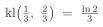
“Monte Carlo gets a quadratic quantum speedup.”
Today we’ll introduce how Monte Carlo rollouts can be used in a quantum computer to solve problems ranging from vaccine distribution to finding an optimal move in a board game.
The typical flow is: choose valid actions, simulate random changes, and evaluate the outcome.
The quantum timing discussion assumes a fault-tolerant computer.
Goal: at most 2 infected after 6 steps.
People are physically located on a grid. Infected individuals may spread the infection to nearby folks.
Suppose we can vaccinate at A or B. Which choice gives us a better chance of keeping the infected count low?
We would need many runs to estimate either choice’s success probability.
One simulated future is a rollout. Later actions follow a fixed policy.
One simulated future is a rollout.
The payoff will be an estimate rather than the exact success probability.
The same idea appears in many planning problems. All you need is to define the valid actions, random updates, and score.
Does the best classical method still need samples?
Does getting enough precision take most of the work?
Can we build an oracle at a reasonable cost?
We’ll check each problem against these questions.
One event and illustrative final counts shown. Repeat updates to H before scoring.
Here is the connection to the game we’ll use, called Sway.
Both examples have a changing state, actions whose validity depends on that state, random transitions, and a final test.
Sway is a board game like Go. In Sway, the winner is the one with the most pieces on the board. After every round, the outcome of a dice roll flips the colors of the pieces, based on similar neighboring colors.
Sway has two players placing stones on a grid. Random events can change a stone’s color, and friendly neighbors reduce that chance.
The board and dice are all we need for this introduction. Behind the scenes, a rate-limited comparison starts sampling two candidate first moves. We’ll introduce those choices and show their estimates after explaining the rules.
Black places a stone, then White places one.
Every stone rolls a twenty-sided die.
An orange die marks a stone that will change color, and all changes happen together.
The board game continues until the board fills.
Here we use a fixed number of rounds so the circuit has a fixed shape.
A stone with no friendly neighbors flips on four of the twenty die faces.
Each friendly neighbor removes one of those faces. With four friendly neighbors, it stays its color.
Edge and corner cells have fewer neighbors, so they always have some chance of flipping.
On the left, every stone uses the board as it was at the start of the event. We apply all color changes together.
On the right, updating one stone early changes the neighbor count for the next stone. That gives a different result with the same dice. In Lesson 4, we’ll make sure our circuit preserves the original board while computing the updates.
Our objective: win probability. Winning by 1 or 10 both return 1.
We stop after a fixed number of rounds and count the stones.
Black gets an outcome of 1 only if it has more stones than White. Ties count as 0.
Fix the first move, then simulate the remaining rounds.
At the end, record the payoff bit.
Reset the board and repeat with fresh random choices.
The average estimates Black’s win probability under this policy.
Each possible first move is one candidate action, also called an arm.
It’s Black’s turn. Which of these three moves would you choose?
Neighbor counts give us a guess. The estimates help us check it, though two of the intervals still overlap.
We choose a tolerance ε. Any action within ε of the best value is acceptable.
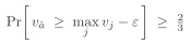
The selector’s guarantee is to return such an action with probability at least two thirds; higher confidence requires extra work.
If we need the unique winner, ε must be smaller than its gap to the runner-up. Otherwise, either of two close moves may be good enough.
These two estimates compare candidate first moves A and B from the same starting board.
For each candidate we run separate futures and estimate the chance that Black finishes ahead.
Next we’ll compare these live estimates with a larger, seeded sample.
These estimates use 400,000 rollouts per move. The easy pair has an estimated gap near 0.04. The closer pair is about 0.006 apart.
We use g for the gap and ε for our chosen tolerance. With ε = 0.003, only the leading move among these candidates qualifies if the estimated gap holds.
The circuit stores random choices in qubits and computes the payoff without measuring.
Call that circuit A. We also need its inverse, A†, which undoes the computation.
Amplitude estimation uses both directions to estimate the payoff probability.
We can group the losing paths along one axis and the winning paths along the other.
Here, x and y are amplitudes. Their squares give the loss and win probabilities, so x² + y² = 1. That puts the state on this circle.
The angle θ tells us the win probability: a = sin²θ. If we can estimate θ, we can calculate a.
Reflect across the x axis (the losing axis), and inspect the mirror image.
Reflect across the initial state.
Together, those reflections rotate the state by 2θ. We call this operation Q.
Q uses A and A†, along with the reflections shown here.
We can implement these operations even when the original win probability is unknown.
For a worked example, a = 1/4 gives θ = 30°. One Q takes the state to 90°. We choose a known angle here so we can check the geometry.
The first advance changes the previous example’s angle to θ = 10°.
Each Q adds 20°: one, two, and four applications reach 30°, 50°, and 90°. Eight overshoot to 170°, where a win is read only 3% of the time.
The state never settles on the winning axis. The odds rise and fall, and the rate of that wave is what we estimate.
Each row starts with a fresh preparation. Each Q costs a rollout forward and backward; measuring the payoff gives one result.
Think of two possible values for the unknown probability.
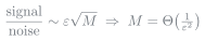
On the left, sampling uncertainty shrinks roughly as 1/√M.
On the right, a small difference in rotation accumulates across coherent queries.
The diagram illustrates the scaling near these probabilities.
Reaching error ε takes order 1/ε² classical samples or 1/ε coherent queries at fixed confidence.
The next slide explains how we read an estimate.
Fresh preparation for every shot. Measure only after the coherent sequence.
Illustrative batches · 512 shots each · Iterative Quantum Amplitude Estimation
Iterative amplitude estimation chooses how many times to apply Q, then measures the payoff bit. We repeat that circuit to estimate its outcome probability and narrow the possible values of θ.
IQAE keeps the near-quadratic query improvement, up to logarithmic factors.
The algorithm needs a bounded payoff, a coherent circuit A, and its inverse.
Random choices must be prepared inside the circuit, and measurements must wait until the coherent sequence finishes.
An ordinary sampling service gives us a bounded result, but it doesn’t provide the circuit access we need.
In Go, the same move from the same position always gives the same next position. Monte Carlo tree search introduces randomness as a way to explore that tree.
Classical methods can also use pruning, learned move preferences, and value estimates. We would need to compare against those before claiming a speedup from fewer rollouts. For this course, we set Go aside at Question 1. Other quantum approaches to game trees need their own analysis.
Imagine two slot-machine arms with win probabilities 1/2 and 1/2 + ε. We want to find the better arm by pulling them.
When ε is small, distinguishing them takes order 1/ε² pulls per arm. This gives us a sampling problem where precision can be expensive. Arms with a large gap are much easier to compare.
An ordinary arm gives us a fresh result each time we pull it. The interface supplies no way to apply A†.
A reversible reward circuit would provide a different kind of access, and the quantum algorithm could use it.
We have explained how to estimate one action’s value. Finding a good action among k candidates adds another layer.
The quantum best-arm construction combines amplitude estimation with a search over candidates. The rings show the cost of that search, the estimates it needs, and the rollout circuit inside each estimate.
The coherent best-arm construction uses roughly √k/ε oracle calls, with logarithmic factors hidden by the tilde. The appendix gives the corresponding classical sampling lower bound for a hard family.
This is a bound for the full selection algorithm under its access assumptions. The interval-based readout we just saw explains probability estimation; the coherent selection wrapper also has to meet its own requirements.
Runtime depends on the cost of implementing each call.
Does sampling remain expensive after the classical shortcuts?
Enumerate outcomes or reuse repeated states. Check sampled answers against exact values.
Try structure, approximations, and ways to reduce variance. Count their cost and error.
Measure whether sampling still dominates at the precision the decision needs.
Randomness and a large tree alone don't establish a sampling lower bound. The appendix gives a bound for a specific access model and hard family.
Small Sway boards can be enumerated exactly. Larger instances need a comparison against the strongest classical methods we can use.
A large number of possible futures motivates sampling, but doesn’t prove that sampling is necessary. The hard-family theorem in the appendix has specific assumptions. Each application still needs this check.
The structure carries over. State encoding and gate costs depend on the model.
Course paper · two implementations
The model supplies three operations: identify valid actions, update the state, and evaluate the outcome. Advance to replace those three pieces one at a time. The outer circuit structure stays visible while the model-specific operations change.
The circuit design has common work around them: decode action choices, keep randomness in registers, preserve enough information to reverse updates, and clear temporary work.
The epidemic model has a different transition rule and payoff, so its resource counts differ too.
Two small oracle implementations have been checked.
| 3×3 · 2 rounds | Sway | Epidemic model |
|---|---|---|
| Qubits | 169 | 146 |
| Gates | 9,768 | 6,472 |
| Sampled payoff | 0.281 ± 0.028 | 0.883 ± 0.020 |
| Exact payoff | 0.271 | 0.891 |
Tested branches agree with the classical simulations. Aggregate estimates agree with exact enumeration.
Course paper, Table I · published validation instances, separate from the live illustration · gate counts before decomposition and error-correction overhead
On small instances, the tested branches agree with classical rollouts, and aggregate results agree with exact enumeration.
This is evidence that the construction carries across models.
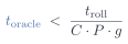
For a separate timing scenario, assume a gap of 0.0001, five milliseconds per classical rollout, and overhead C = 10. This is a fixed pairwise comparison; it omits the search among k actions.
The model gives 5.8 days on one core or 8.3 minutes on a thousand cores with perfect scaling. A coherent call must take less than five milliseconds to beat the latter.
At one millisecond per call, the quantum estimate is 100 seconds. At 100 milliseconds, it is 2.8 hours. The gap and timings are assumptions, separate from the measured 5×5 example.
| Example | What we learned | Next step |
|---|---|---|
| Go | Rollouts are one classical approach. | Compare against stronger classical methods. |
| Sampled bandit | Close arms need many samples; the interface lacks A†. | Coherent access would need a different implementation. |
| Sway + epidemic | The shared oracle structure has two implementations. | Build the components and count their costs. |
We have a reusable construction to study. A runtime advantage still depends on the instance and hardware costs.
The construction applies when we can implement valid-action selection, stochastic transitions, and payoff evaluation reversibly at a manageable cost.
Sway gives us a small example to learn on. The epidemic implementation shows how those pieces change in another model.
For a new application, we still check the classical alternatives, the required precision, and the cost of the quantum circuit.
Let’s look inside one oracle call. We need qubits for the board, move selection, dice, temporary work, and the payoff.
In Lesson 3, we’ll build those pieces into a circuit.
Next: build one rollout circuit.
We'll implement the board, legal-move selection, random choices, and payoff in Lesson 3.
Continue to Lesson 3 Optional proof and readout detailsContinue to Lesson 3 to build the rollout circuit. The remaining slides are optional: the sampling lower bound, assumptions behind the theorem, an alternative readout, and larger resource counts.
To prove a lower bound, we construct several similar problems with different best arms.
In the starting problem, arm zero wins with probability 1/2 + 4ε. All other arms win with probability 1/2. In problem j, we raise arm j to 1/2 + 6ε, making it the winner.
Each pull gives only a little evidence about whether an arm’s probability has changed. In this construction, that information is at most 96ε² per pull.
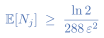
The proof requires at least ln(2)/3 total evidence. Dividing gives a lower bound of ln(2)/(288ε²) expected pulls per contender. The constant is machine-checked, and the bound also covers algorithms that choose their next arm based on earlier results.
Any contender could be the arm whose probability changed. An algorithm that works across the whole family has to check each one.
There are k − 1 contenders, each requiring order 1/ε² pulls. Adding them gives the classical lower bound for this sampling model.
| proven | Õ(√k/ε) upper bound · Ω(k/ε²) lower bound on the hard family |
| proven, robustness | the hard instance recurs across an exponential family (bounded influence) |
| assumed | coherent access: A, A†, no measurement inside |
| not included | unrestricted classical structure · FT overhead · wall clock |
We have a quantum upper bound and a classical lower bound for the constructed family, each under its stated access model.
The robustness result allows factors to vary when their combined influence stays below ε. The best action stays the same across those configurations. Under the modularity assumption, the lower bound extends too.
Coherent access is an assumption. Classical shortcuts, error-correction costs, and runtime still need separate checks. Lessons 3 and 4 build the oracle.
The original amplitude-estimation circuit uses controlled powers of Q and an inverse Fourier transform. Measurement yields a phase estimate, which determines the payoff probability.
This is an alternative to the iterative readout in the main lesson. It introduces an extra phase register.
Hold a stone’s friendly-neighbor count fixed. With flip probability p, its expected contribution to the color margin is multiplied by 1 − 2p per event.
For two friends, that factor is 0.8, and 0.8⁴⁰ is about 0.00013. This calculation concerns an expected color margin. It does not determine the gap between two moves’ win probabilities on a full board.
Neighbor counts change during the game. We measure action-value gaps separately.
Back to Lesson 3 and course links
These are circuit counts before gate decomposition and error-correction overhead. The small validation cases and the larger compiled-only cases are shown separately.
A 20×20 Sway board over ten rounds uses about six million gates in this implementation. Converting that count into time requires a hardware model.